Pixel-Space Diffusion Is Back: What Changed and How to Evaluate It

For five years almost every serious image generator has worked in a compressed latent space, behind a separately trained autoencoder. A run of papers from 2024 to October 2026 shows that diffusion directly on pixels can now compete, and also shows exactly where it still falls short. This post explains what changed, corrects a common mix-up about which models are actually pixel-space, and gives you a concrete way to test the trade-off on your own data.
Why latent diffusion became the default
A diffusion model learns to turn noise into an image by removing a little noise at a time. Doing that directly on a 1024×1024 RGB image means processing about three million numbers at every step. Rombach and colleagues' latent diffusion paper (CVPR 2022) side-stepped this by training the diffusion model in the latent space of a pretrained autoencoder, which they describe as reaching "a near-optimal point between complexity reduction and detail preservation" and which made training feasible on far less hardware [1].
The Diffusion Transformer (DiT) paper shows the arithmetic. It uses the Stable Diffusion VAE, which downsamples by a factor of 8, so a 256×256×3 image becomes a 32×32×4 latent. Cut into 2×2 patches, that is 256 tokens for the transformer [2].
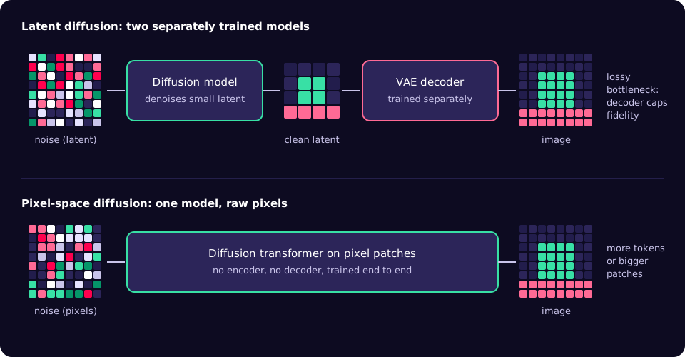
The cost of the trick is that the autoencoder is a separate model with its own training run, and the final image can never be better than what its decoder can reconstruct. That "lossy latent bottleneck" is precisely what the newer pixel-space work tries to remove [6].
What changed: four results worth knowing
| Work | What it showed |
|---|---|
| Hourglass Diffusion Transformer, HDiT (ICML 2024) [3] | A hierarchical transformer whose cost scales linearly with pixel count. Trains without multiscale architectures, latent autoencoders or self-conditioning; competitive on ImageNet-256 and a new state of the art for diffusion models on FFHQ-1024. |
| Simpler Diffusion, SiD2 (CVPR 2025) [4] | Pixel-space diffusion reaching 1.5 FID on ImageNet 512×512, with the authors arguing pixel models can match latent ones in both quality and efficiency. |
| JiT, "Back to Basics" (Li and He, 2025) [5] | Plain transformers with large 16- or 32-pixel patches on raw pixels, with no tokenizer, no pre-training and no extra loss, made to work by predicting the clean image instead of the noise. |
| MFlow and ConvRefiner (Mukhopadhyay et al., October 2026) [6] | Revisits JiT's choice of target, finds that the best target depends on data representation and model size, and identifies a persistent high-frequency deficit in pixel diffusion transformers, with a post-hoc fix. |
One HDiT number is often quoted loosely. Its project page reports that at megapixel resolution HDiT-B/4 needs less than 1% of the compute of a comparable-size DiT run in pixel space [3]. That is a comparison against a naive pixel transformer, not against a latent pipeline, so it does not mean pixel diffusion is now a hundred times cheaper than latent diffusion.
Why predicting the clean image matters
A diffusion network can be trained to output one of several targets at each step: the noise that was added (often written ε), the "velocity" between noise and image (u), or the clean image itself (x0). Mathematically they are interchangeable, but they are not equally easy to learn.
Look at the token arithmetic. At 256×256 with 16×16 patches, a pixel transformer also sees 256 tokens, the same sequence length as DiT on its latent. The difference is that each token now carries 16×16×3 = 768 numbers instead of 2×2×4 = 16.
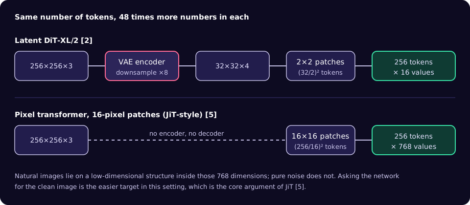
Li and He's argument is that natural images sit on a low-dimensional manifold while noise does not, so a network with apparently too little capacity for 768-dimensional tokens can still predict the clean image well; asking it to predict noise in that setting "can fail catastrophically" [5]. The October 2026 MFlow paper refines this: it learns to interpolate between clean-image and velocity prediction, and finds the preference shifts with data representation and model capacity, with larger models leaning back towards velocity prediction [6]. Practical reading: the target is a design choice to test at your model size, not a settled rule.
The catch: a high-frequency deficit
The same paper reports that vanilla pixel diffusion transformers, whatever their prediction target, "retain a persistent high-frequency deficit relative to real images" [6]. High frequencies in an image are the fast changes: sharp edges, fine texture, small text. In the frequency spectrum, the generated images carry less power at the top end than real ones.
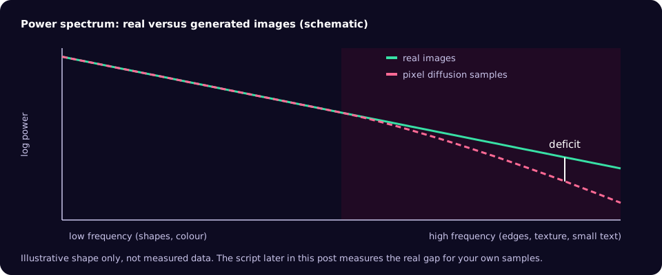
Their remedy, ConvRefiner, is a small convolutional module trained afterwards with an adversarial loss while the diffusion backbone stays frozen; with a small amount of extra training it restores the high-frequency statistics "while preserving FID" [6]. Note what that implies: removing the autoencoder does not automatically give you crisper output. Latent models lose detail at the decoder; pixel models can lose it in the generator. You need to measure both.
A correction: Sana is a latent model
NVIDIA's Sana is sometimes listed alongside pixel-space models because it is fast at high resolution. It is not pixel-space. Sana uses a deep-compression autoencoder that compresses images 32×, rather than the usual 8×, to cut the number of latent tokens. That is how it reaches 4096×4096 output and how Sana-0.6B generates a 1024×1024 image in under a second on a 16 GB laptop GPU [7]. It is a strong reminder that the latent side is also moving: deeper compression is the competing answer to the same compute problem.
Pixel-space and latent diffusion compared
| Latent diffusion | Pixel-space diffusion | |
|---|---|---|
| Models to train and version | Autoencoder plus diffusion model | One diffusion model (plus an optional refiner) |
| Quality ceiling | Bounded by the decoder's reconstruction | No decoder bound; can show a high-frequency deficit [6] |
| Compute per step | Low: tokens come from a compressed latent | Higher, unless the architecture compensates (hierarchy, large patches) [3][5] |
| Ecosystem today | Mature: most open text-to-image models and tooling | Mostly research code and class-conditional benchmarks |
| Best evidence | Production systems such as Sana [7] | Strong ImageNet results such as SiD2 at 1.5 FID [4] |
Playbook: testing pixel versus latent on your problem
If you train or fine-tune image models for a specific domain (product imagery, documents, scientific or industrial images), here is a sequence that turns the debate into measurements.
- Fix the task and the metrics first. Class-conditional or text-to-image? Pick metrics before running anything: FID for distribution match, a text-alignment benchmark such as GenEval for prompts, and a domain check that matters to you (for example, can a human read the small text).
- Measure the autoencoder ceiling. Encode and decode a held-out set of your real images with the VAE you would use and compute reconstruction quality (rFID, PSNR, SSIM, LPIPS). If reconstruction already destroys the detail you care about, no latent model trained on top can bring it back.
- Estimate compute from token counts. Work out tokens per image and values per token for each option at your target resolution, as in the figure above. Transformer cost grows quickly with sequence length, so this predicts where pixel models get expensive.
- Train matched baselines in one codebase. DiffusionBench is an open, unified codebase that trains and evaluates diffusion transformers across VAE, representation-autoencoder (RAE) and pixel-space configurations, with FID/IS for ImageNet and GenEval, DPGBench, GenAIBench and VQAScore for text-to-image [8]. Using one codebase removes most of the "different training recipe" noise from the comparison.
- Measure the spectrum, not only FID. Compare the radially averaged power spectrum of generated and real images (script below). A ratio well under 1 at high frequencies is the deficit described above.
- If pixel wins on fidelity but lacks detail, test a refiner. A post-hoc refiner on a frozen backbone is cheaper than retraining [6].
- Decide with the whole bill. Training GPU-hours, inference latency at your resolution, number of models to version, and the domain check from step 1.
Running DiffusionBench
These commands are from the project README [8]. Training uses 8 GPUs per node by default, and the README expects Weights & Biases variables to be set; pick the Stage 2 config for the pixel or VAE family you are testing.
# install dependencies (uv)
uv sync

# prepare data and download released checkpoints
uv run python scripts/prepare.py --data {all,imagenet,t2i,t2i-res512,eval}
uv run hf download diffusion-bench/diffusion-bench --local-dir pretrained_models --exclude .gitattributes

# Stage 2: train a diffusion model (VAE, RAE or pixel config)
uv run torchrun --standalone --nproc_per_node=8 src/train.py \
  --config [STAGE2_CONFIG_PATH] --results-dir results/stage2 --precision bf16 --compile --wandb

# Stage 2 generation eval (FID/IS, GenEval, DPGBench, ...)
uv run torchrun --nproc_per_node=8 src/offline_eval.py --config [STAGE2_CONFIG_PATH]
Measuring the high-frequency gap
This short script compares the average spectrum of two folders of same-sized square images. It needs only NumPy and Pillow. A ratio of 1.0 means your samples match real images at high frequencies.
import glob
import sys

import numpy as np
from PIL import Image


def radial_power(path):
    """Radially averaged power spectrum of one greyscale, square image."""
    x = np.asarray(Image.open(path).convert("L"), dtype=np.float64) / 255.0
    h, w = x.shape
    assert h == w, f"{path}: crop to a square first"
    x = x - x.mean()
    power = np.abs(np.fft.fftshift(np.fft.fft2(x))) ** 2
    yy, xx = np.indices(power.shape)
    r = np.hypot(yy - h // 2, xx - w // 2).astype(int)
    radial = np.bincount(r.ravel(), power.ravel()) / np.bincount(r.ravel())
    return radial[: h // 2]


def mean_spectrum(pattern):
    paths = sorted(glob.glob(pattern))
    return np.mean([radial_power(p) for p in paths], axis=0)


real = mean_spectrum(sys.argv[1])   # e.g. "real/*.png"
fake = mean_spectrum(sys.argv[2])   # e.g. "generated/*.png", same resolution
ratio = fake / real                 # 1.0 means "matches real images"
top = slice(len(ratio) * 3 // 4, None)
print(f"high-frequency power ratio (top quarter): {ratio[top].mean():.3f}")
Run it as python spectrum_gap.py "real/*.png" "generated/*.png". Use a few hundred images per side and the same resolution and file format for both, since JPEG compression itself removes high frequencies.
Checklist
- Task, resolution and metrics are written down before any training.
- Autoencoder reconstruction quality is measured on your own images.
- Token counts and values per token are calculated for each candidate.
- Pixel and latent baselines share one codebase and training budget.
- Spectrum ratio is reported next to FID for every candidate.
- Inference latency is measured at the real target resolution and batch size.
- Every model in the pipeline (VAE, backbone, refiner) is versioned with its training data.
Common mistakes
- Calling a fast high-resolution model "pixel-space". Check for an autoencoder. Sana, for example, is latent [7].
- Reading the HDiT "under 1%" figure as a saving over latent diffusion. It is relative to a pixel-space DiT [3].
- Trusting FID alone. A model can preserve FID and still lack high-frequency detail; that is exactly the case ConvRefiner targets [6].
- Assuming no autoencoder means sharper images. The detail can be lost in the generator instead of the decoder.
- Comparing models trained with different recipes and budgets. You end up measuring the recipe, not the representation.
- Copying a prediction target from a paper at a different model size. The preferred target changes with capacity [6].
What to do this week
- List the image models in your stack and note for each whether it uses an autoencoder, and which one.
- Run 200 of your real images through that autoencoder and look at the reconstructions next to the originals, especially edges and small text.
- Run the spectrum script on real images versus your current model's output to get a baseline number.
- Clone DiffusionBench and read through its pixel and VAE Stage 2 configs to size a matched experiment.
- Write a one-page decision note: what result would make you switch, and what it would cost in GPU hours.
Pixel-space diffusion is a real option again, but the decision is an engineering one about where detail is lost and what compute you can afford. If you are planning that kind of training or evaluation run and need the GPU capacity to do it properly, see our GPU clusters page.
References
- Rombach et al., "High-Resolution Image Synthesis with Latent Diffusion Models", CVPR 2022, arXiv:2112.10752
- Peebles and Xie, "Scalable Diffusion Models with Transformers" (DiT), arXiv:2212.09748
- Crowson et al., "Scalable High-Resolution Pixel-Space Image Synthesis with Hourglass Diffusion Transformers", ICML 2024, project page (arXiv:2401.11605)
- Hoogeboom et al., "Simpler Diffusion (SiD2): 1.5 FID on ImageNet512 with pixel-space diffusion", CVPR 2025, arXiv:2410.19324
- Li and He, "Back to Basics: Let Denoising Generative Models Denoise" (JiT), arXiv:2511.13720
- Mukhopadhyay, Mai, Shrivastava and Mahapatra, "Rethinking the design space of Vanilla Pixel Diffusion Transformers", arXiv:2610.23854, October 2026
- Xie et al., "SANA: Efficient High-Resolution Image Synthesis with Linear Diffusion Transformers", NVIDIA project page (arXiv:2410.10629)
- End2End-Diffusion, DiffusionBench repository, GitHub